Notebook initialization

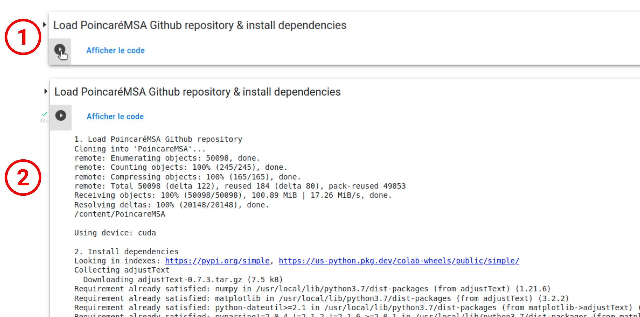
To execute code on the Notebook, one simply need to click on the "execute" button (1). The initialization step will first download the required stripts from the GitHub repository and load Python modules.

Data upload

You can provide input for PoincaréMSA in three different ways:

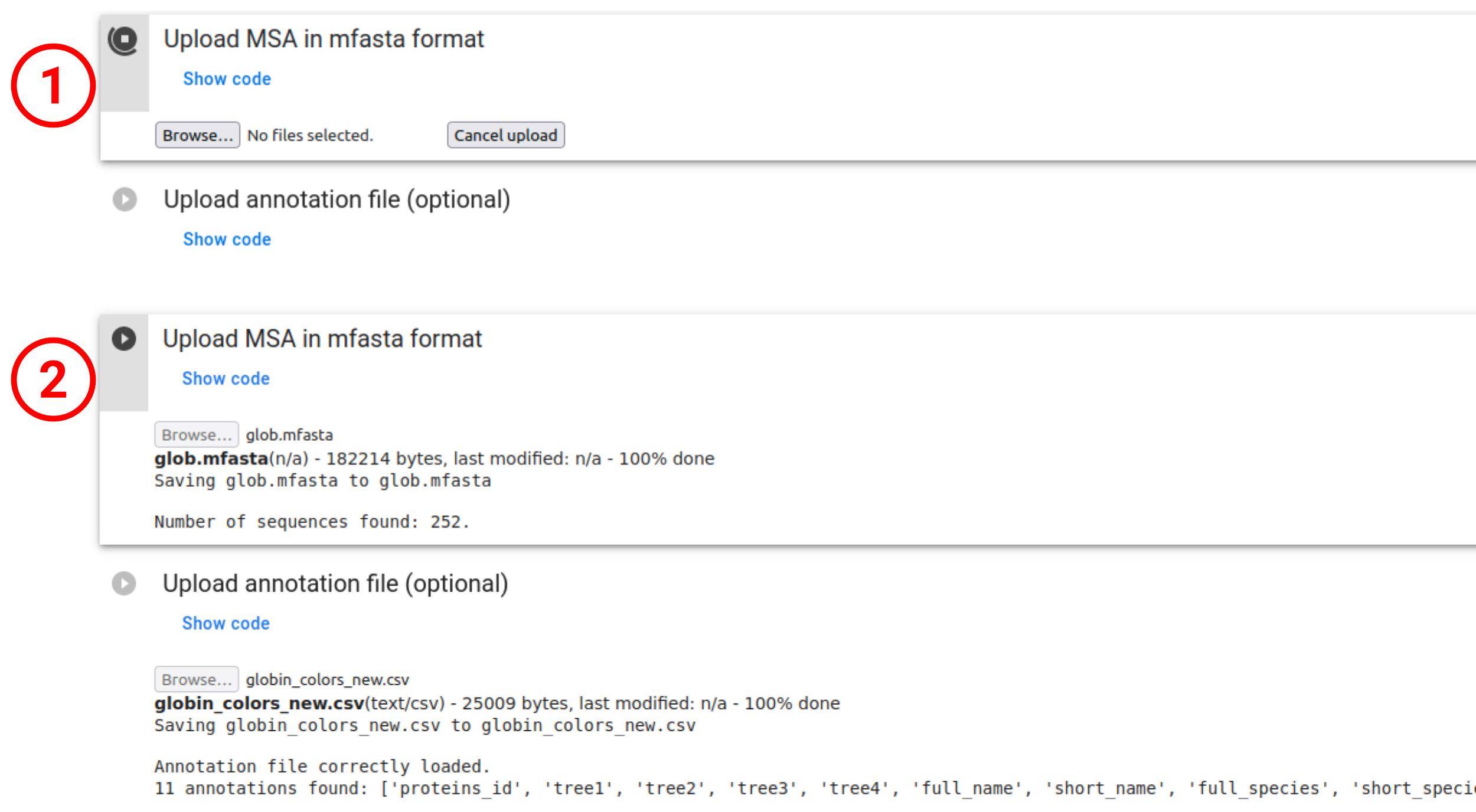
1. To project a user-defined protein family, please prepare your MSA in multi-fasta (.mfasta) format and use PoincareMSA_colab.ipynb. You can also provide an annotation file to color resulting projections in .csv format with columns name as the first row, and each other row corresponding to a protein in the .mfasta file in the same order. The user ca also provide a list of UniProt IDs to create an annotation file automatically.
2. To launch examples of globin, kinase or thioredoxin family with corresponding annotations, please use PoincareMSA_colab_examples.ipynb, which automatically uploads all necessary data from examples directory on github.
3. To build your alignment from a given target sequence, please use PoincareMSA_colab_MMseqs2.ipynb. In this case, annotation for coloring will be built automatically using information available in UniProt.

Data preparation

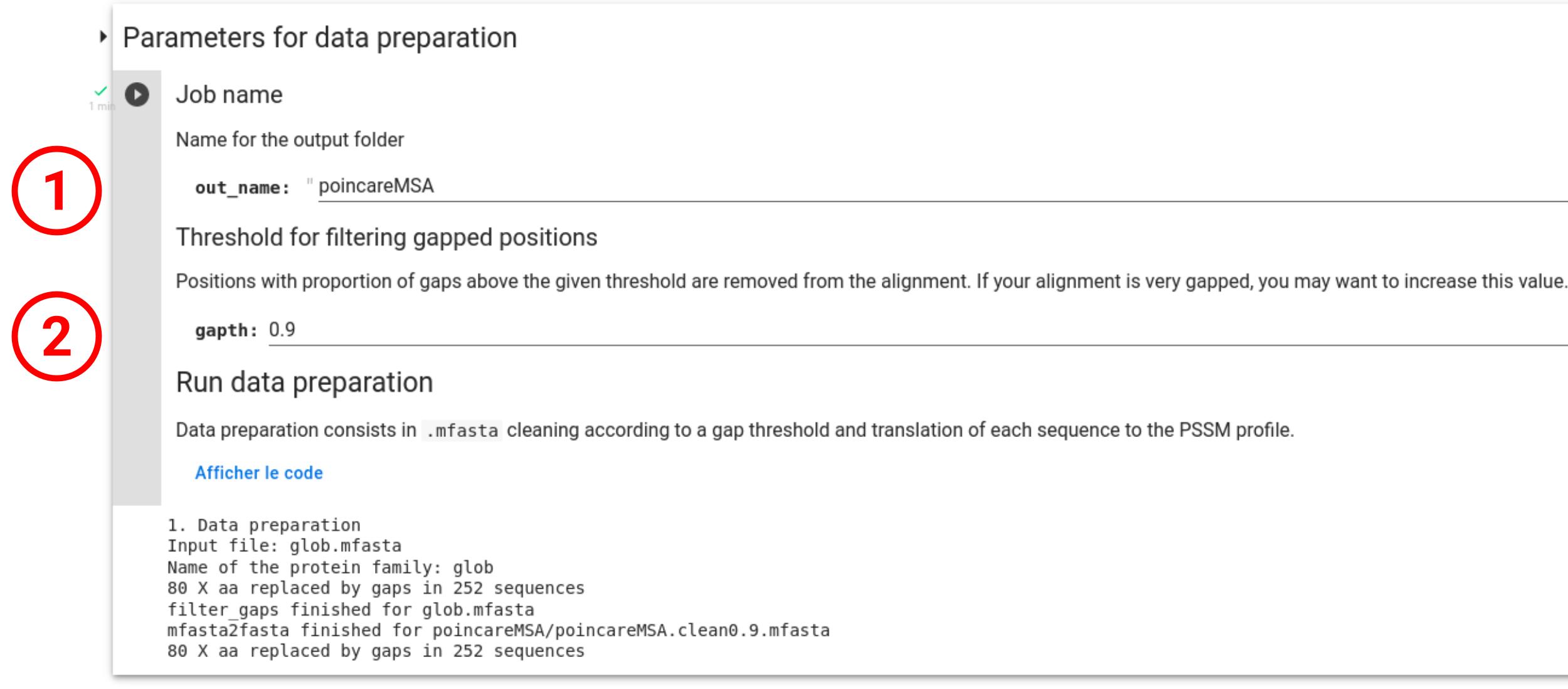
The "Parameters for data prepartation" section allows to select the name of the intermediate data folder (1) as well as tuning the MSA filtering parameter (2). For more detail about this parameter, see Klimovskaia et al..

Data projection using Poincaré disk

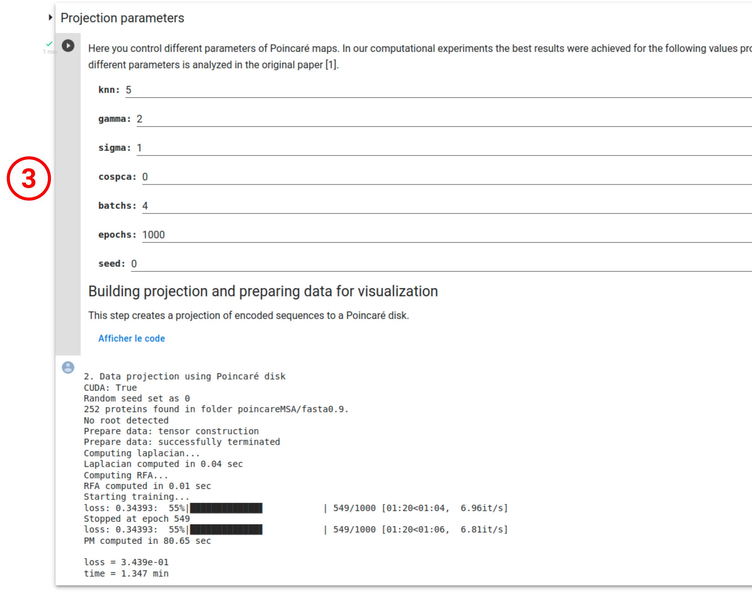
During this step, the encoded MSA will be projected into the Poincaré disk according to the default parameters (3) already specified (see Klimovskaia et al. for more details). It is important to note that the projection step is nondetermenistic, i.e it's results may vary depending on the PyTorch release, the execution platform, or between CPU and GPU executions, even when using identical seeds.

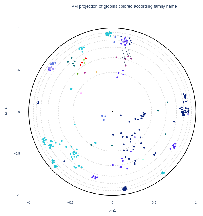
Projection visualization

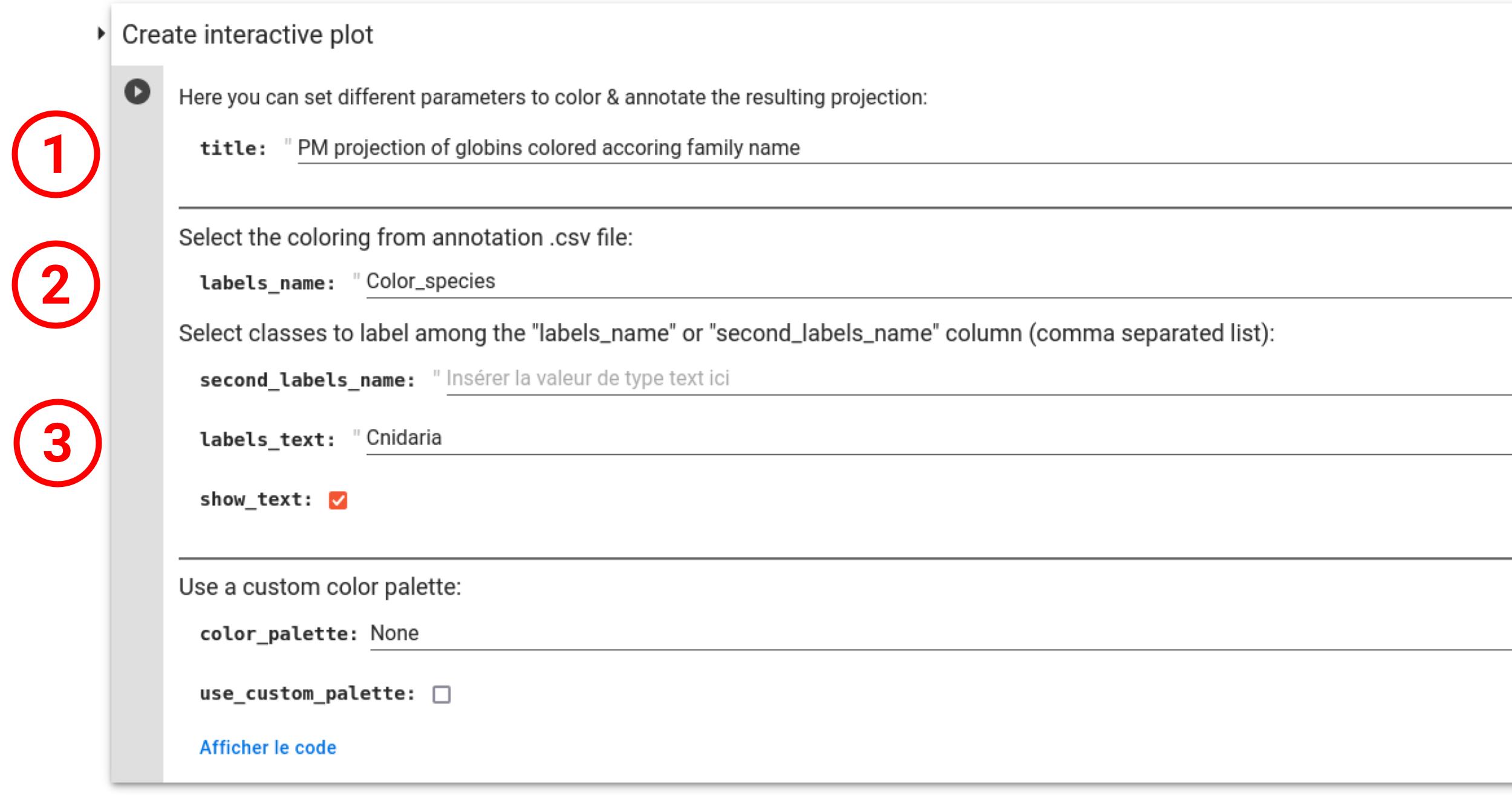
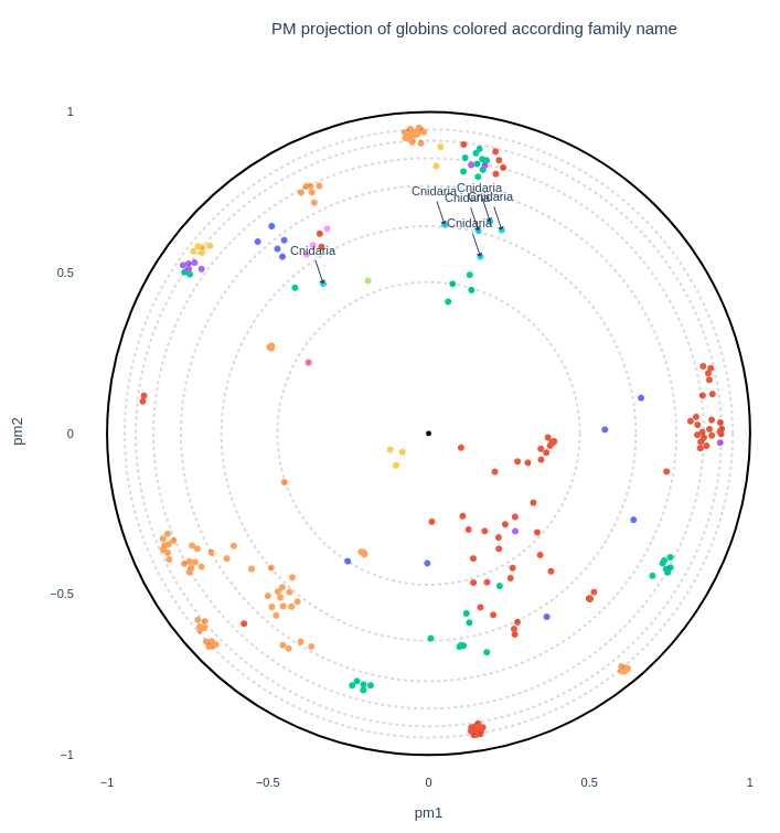
Once the input MSA has been correctly processed, user can presonalize the projection visualization with a title to the plot (1), and with annotation colors and text if a .csv file has been provided. The color of the markers can be selected with the "labels_name" field (2). In addition, user can add text labels on the plot, in order to lay the emphasis on a class or a group of classes (list of labels separated by commas. ex: Artrhopoda, Cnidaria) from the "labels_name" column (3). If the "second_labels_name" field is used (5), the "labels_text" plot annotations will be selected in this column instead of the "labels_name" one used for coloring, allowing more complex representations.

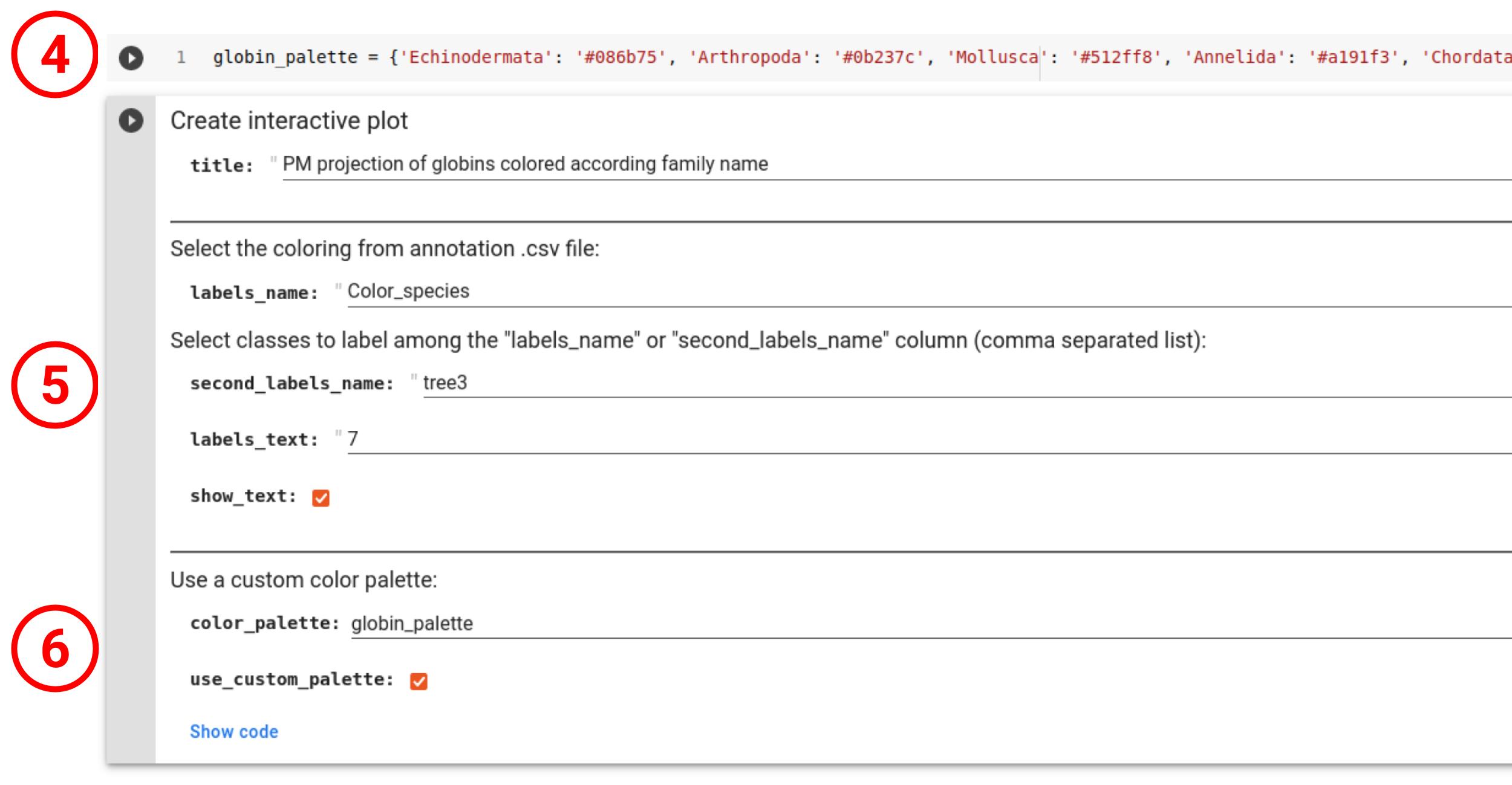
User can also manually create a custom color palette in the form of a Python dictionnary in which the keys are row values of the coloring column ("labels_name") and the values are colors (4). The variable name used for this dictionnary can then be inputed in the "color_palette" field to be used in the plot (6).

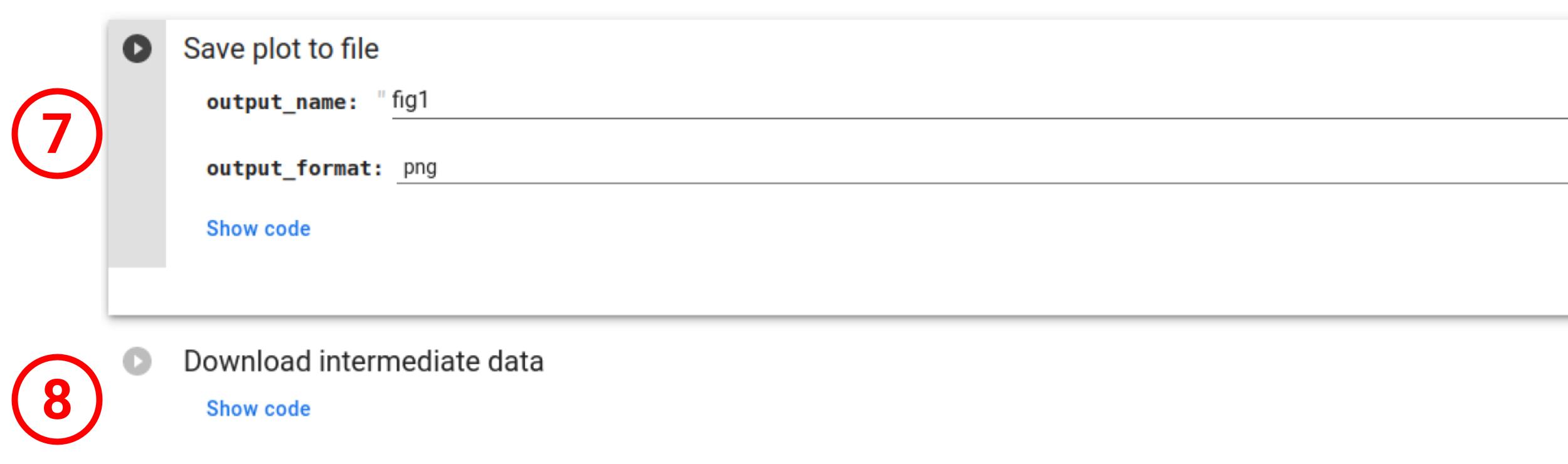
One can also download the plot in .png, .pdf, .html (interactive) or .svg (7) as well as downloading all the intermediate data in a .zip achive (8).